Introduction
One of the primary formulae you may require in your spreadsheet is to calculate an average. There are many methods to average numbers or cells in Google Sheets.
You may use Google Sheets to keep track of your pupils’ grades or your company’s revenue. When you want to acquire an average of a set of cells, particular values, or a mix of both, you have many methods to choose from. Let’s take a closer look.
Look at a Quick Average
Google Sheets has a few computations that are visible at a glance. This is perfect if you don’t want to put the average of your cells on your sheet but just want to observe it.
Choose the cells that contain the numbers you wish to average. Then, in Google Sheets, look down in the bottom right corner. You’ll see a box with a simple computation, most likely Sum.
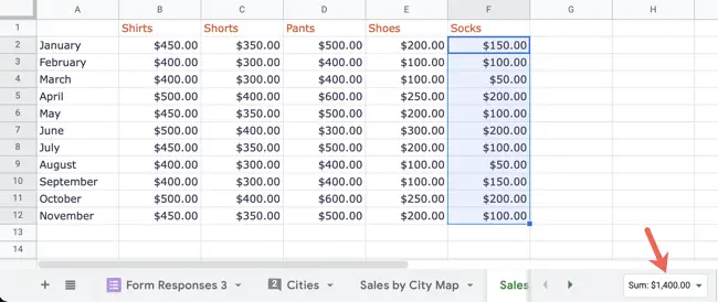
When you click the arrow to examine the other alternatives, you’ll see the average.
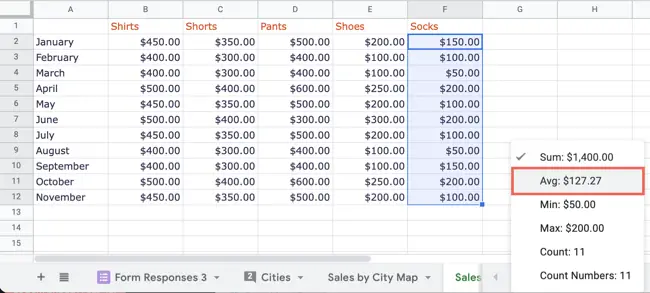
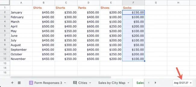
If you want to change your numbers or examine the average for another group of cells, you may retain the average shown in the box by selecting it.
Make use of the Functions Button
You may add the average to your sheet by clicking the Functions icon in the toolbar.
Choose the cells that contain the numbers you wish to average. To examine the available computations, click the arrow next to the Functions icon and choose “Average.”

You’ll find the temporary location for the function at the bottom of a column or the furthest right of a row. Confirm that the range specified in the formula is accurate, and then hit Enter or Return.

The average formula is then automatically entered into the cell for you.

Manually Enter the Function
Perhaps you’d want to calculate the average of nonadjacent cells, numbers, or a mix of cells and numbers. In this instance, manually inputting the AVERAGE function is your best bet. This offers you the freedom to modify the formula as needed.
In Google Sheets, the function syntax is AVERAGE(value1, value2,…), where value1 is necessary and value2 is optional.
Choose the cell in which you wish to see the average. For this first example, we’ll average two nonadjacent cell groups, B2 through B12 and E2 through E12. Enter the formula below, substituting the cell references with your own.
=AVERAGE(B2:B12,E2:E12)
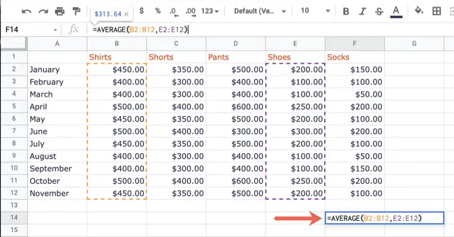
If the numbers you wish to average do not exist inside cells, just insert them into the formula to get their average.
=AVERAGE(5,10,15,20,100,120)

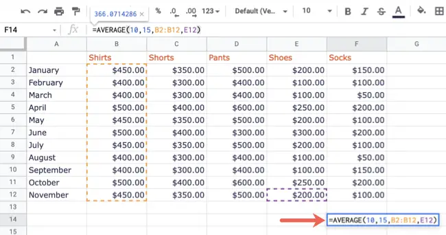
In the formula, you may also mix cells and numbers. We’ll use the following to average numbers 10 and 15, the cell range B2 through B12, and cell E12.
=AVERAGE(10,15,B2:B12,E12)
You may choose the best solution for calculating an average in Google Sheets based on your requirements.
Also, learn how to multiply integers in Google Sheets and how to utilize the MEDIAN function.

