
Introduction
When using Google Sheets to handle financials, you’re certain to come into values that are less than zero. You can make those negative numbers stand out by making them appear in red, which is considerably clearer than a minus sign or parenthesis.
This may be accomplished in one of two ways. You may rapidly apply some custom format settings. If you want greater control, try using a conditional formatting rule.
Using a Custom Format, Color Negative Numbers Red
You may add a red color to a range of cells in Google Sheets by using a custom number format. Only negative numbers will be highlighted in red.
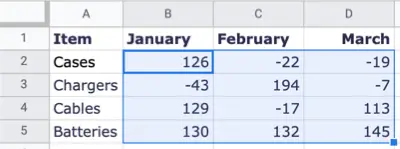
Open your spreadsheet in Google Sheets after signing in if required. Choose the cells that contain or may contain negative numbers.
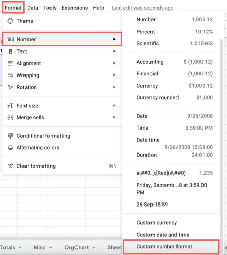
Navigate to the Format tab, then to Number, and finally to “Custom Number Format.”
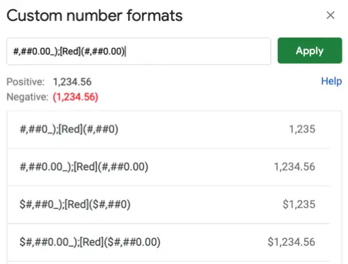
Type “red” into the box at the top of the window that displays. You’ll next be presented with a selection of number formats from which to pick. You may click on each one to get a sample of how it will look. The negative figures are shown in parenthesis with red text in these selections.
When you’ve found the one you’re looking for, click “Apply.”
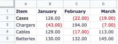
Your chosen cells will then be updated to reflect the new format for negative values. When you modify a value to a positive integer, the custom format changes to remove the parenthesis and red font.
Use Conditional Formatting to make Negative Numbers Red
You may use conditional formatting to change the typeface for negative integers to red without changing the format.
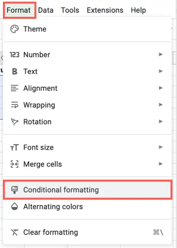
Choose the cell range, then go to the Format tab and choose “Conditional Formatting.” This brings up the right-hand sidebar where you may build your rule.
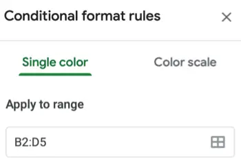
Select the Single Color tab at the top and confirm the cells you’ve chosen in the Apply To Range box. If you choose, you may optionally provide an extra range of cells.
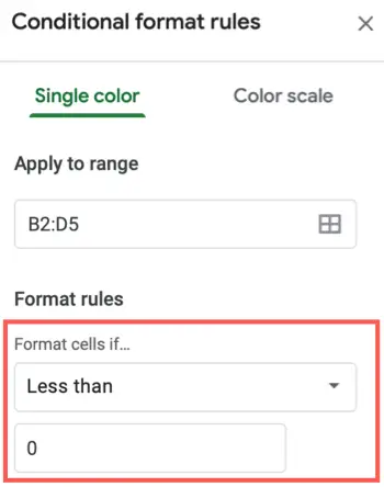
Open the Format Cells If drop-down box in the Format Rules section and pick “Less Than.” Enter a zero in the box just underneath.
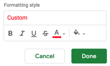
Open the Fill Color palette in the Formatting Style box and choose “None.” Then, open the Text Color palette and choose a red tone. Click the “Done” button.
Your chosen cells will be updated to show negative integers in red while retaining the format you use to identify negative numbers.
If you want to make negative numbers in Google Sheets red, these two simple methods will allow you to set it up and then automatically turn them red as necessary.