
Introduction
Duplicates may arise no matter how carefully you input or import data. While you could detect and eliminate duplicates, you should consider reviewing them rather than removing them. We’ll teach you how to use Google Sheets to spot duplicates.
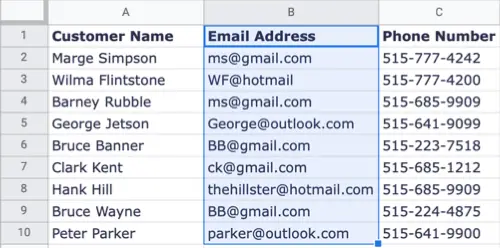
Duplicates should not exist in a list of client email addresses and phone numbers, product IDs and order numbers, or similar data. You may next check and repair the inaccurate data by detecting and marking duplicates in your spreadsheet.
While conditional formatting in Microsoft Excel makes it simple to spot duplicates, Google Sheets does not presently provide this feature. However, spotting duplicates in your sheet may be done in a few clicks using a custom formula in addition to conditional formatting.
Duplicates in Google Sheets may be found by highlighting them
Open Google Sheets and sign in to the spreadsheet you wish to work with. Choose the cells in which you wish to look for duplicates. This may be a cell range, a column, or a row.
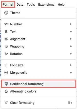
From the menu, choose Format > Conditional Formatting. This brings up the Conditional Formatting sidebar, where you may create a rule that will identify duplicate data.
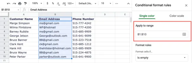
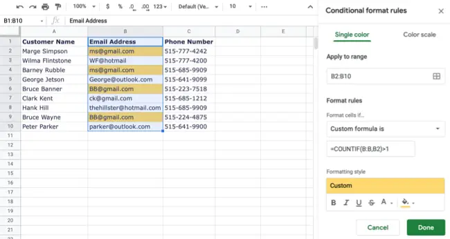
Select the Single Color tab at the top of the sidebar and check the cells under Apply to Range.
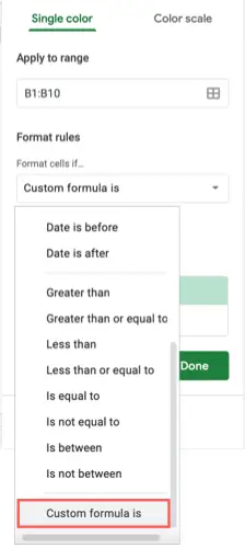
Open the Format Cells If drop-down box underneath Format Rules and choose “Custom Formula Is” from the bottom of the list.
Fill in the Value or Formula box underneath the drop-down box with the following formula. Replace the letters and cell references in the formula with those from the cell range you want to work with.
- =COUNTIF(B:B,B1)>1
COUNTIF is the function, and the range is B:B. (column,) B1 is the criterion, and >1 denotes more than one.
To acquire correct cell references as the range, you may use the formula below.
- =COUNTIF($B$1:$B$10,B1)>1
COUNTIF is the function, $B$1:$B$10 is the range, B1 is the condition, and >1 signifies more than one.
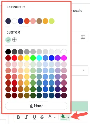
Choose the sort of highlight you wish to use under Formatting Style. The Fill Color icon may be used to choose a color from the palette. If you like, you may use bold, italic, or a color to format the font in the cells.
When you’re finished, click “Done” to apply the conditional formatting rule. The cells containing duplicate data should be formatted in the way you choose.
As you make changes to the duplicate data, the conditional formatting will vanish, leaving you with just the duplicates.
A Conditional Formatting Rule may be edited, added, or removed
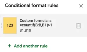
In Google Sheets, you may quickly edit a rule, add a new one, or remove an existing one. Format > Conditional Formatting will open the sidebar. You’ll be able to view the rules you’ve established.
- Select the rule you want to update, make your changes, and then click “Done.”
- Select “Add Another Rule” to create an extra rule.
- Hover your mouse over a rule and click the trash can symbol to delete it.
You may fix incorrect data by detecting and flagging duplicates in Google Sheets. If you’re looking for more methods to utilize conditional formatting in Google Sheets, check out how to apply a value-based color scale or how to highlight blanks or cells with mistakes.
