Introduction

Color may be a great way to make data stand out in Microsoft Excel. So, if you want to count how many cells you’ve colored, you have a few of options.

Perhaps you’ve colored cells to represent sales figures, product numbers, zip codes, or anything else. The following two methods to count those cells work excellent whether you’ve manually used color to highlight cells or their content or you’ve put up a conditional formatting rule to do so.

Use Find to Count Colored Cells

This is the fastest of the two methods for counting colored cells. Because there is no need to include a function or formula, the count will simply be shown for you to view and manually record if desired.

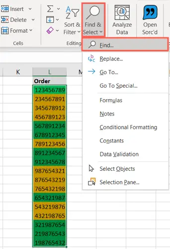
Go to the Home tab after selecting the cells you wish to deal with. Click “Find & Select” in the Editing area of the ribbon and then “Find.”

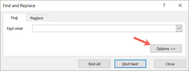
Click “Options” when the Find and Replace box appears.

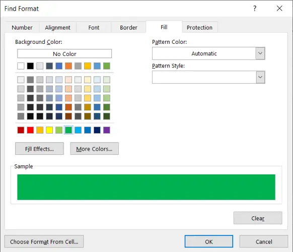
Click “Format” if you know the exact formatting you used for the colored cells, such as a particular green fill. Then, in the Find Format box, pick the color format using the Font, Border, and Fill tabs and click “OK.”

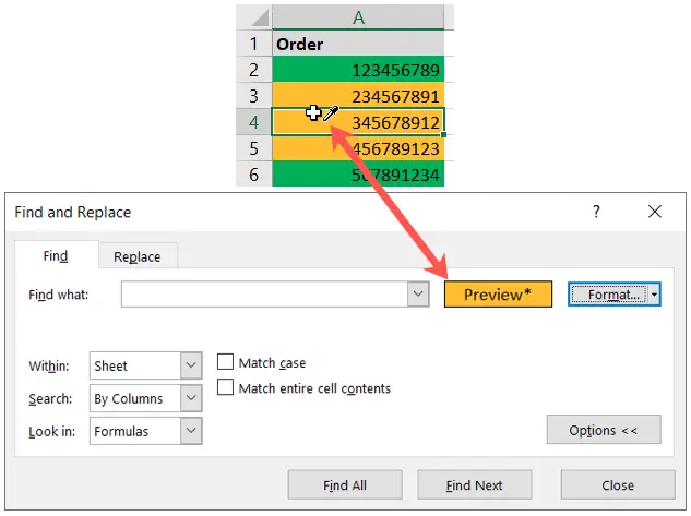
You may use a different method if you’re not sure of the precise color or if you utilized numerous format forms like a fill color, border, and font color. Select “Choose Format From Cell” from the arrow next to the Format button.

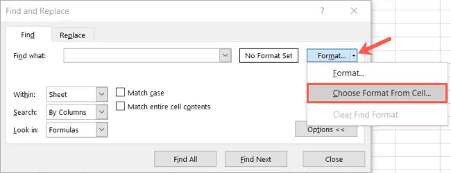
Move your mouse on one of the cells you wish to count and click when it turns into an eyedropper. The formatting for that cell will be shown in the preview.

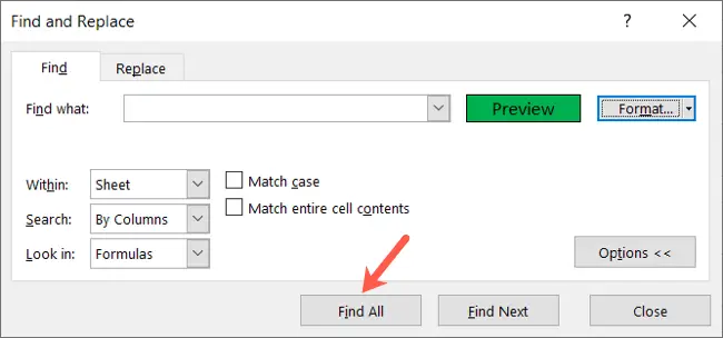
After you’ve entered the format you want using one of the two methods above, you should evaluate your preview. If everything seems to be in order, click “Find All” at the bottom of the window.

When the window expands to show your findings, you’ll notice “X Cell(s) Found” in the bottom left corner. That’s all for your tally!

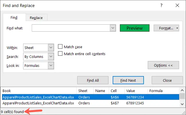
The precise cells may also be seen at the bottom area of the window, right above the cell count.

Using a Filter, Count Colored Cells

This second technique is for you if you want to change the data over time and want to preserve a cell devoted to your colored cell count. You’ll utilize a function and a filter in tandem.

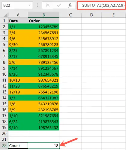
Let’s begin by adding the SUBTOTAL function. Go to the cell where you want your count to appear. Replace the A2:A19 references with those for your own range of cells, and then press Enter.

• =SUBTOTAL(102,A2:A19)

The numerical indicator for the COUNT function is 102 in the formula.

• Note: See the table on Microsoft’s support page for SUBTOTAL for alternative function numbers you may use with the function.

You should see a count of all cells containing data as a fast check to ensure you typed the function properly.

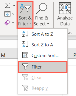
It’s now time to apply the filter to your cells. Go to the Home tab after selecting your column heading. Select “Filter” from the “Sort & Filter” menu.

Each column header now has a filter button (arrow) next to it. Move your pointer to “Filter by Color” and click the one for the column of colored cells you wish to count. In a pop-out menu, you’ll see the colors you’re utilizing, so choose the color you want to count.

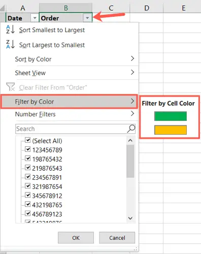
• Note that if you choose font color instead of or in addition to cell color, the pop-out menu will show those choices.

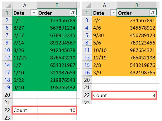
When you look at your subtotal cell, you should see that the count has been reduced to just those cells that correspond to the color you chose. You may also quickly view those counts by returning to the filter button and selecting a different color from the pop-out menu.

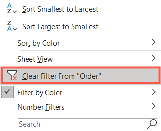
You may clear the filter when you’ve finished obtaining counts with it to view all of your data once again. Select “Clear Filter From” from the filter menu.

If you’re currently using colors in Microsoft Excel, you should know that they may be used for more than simply making data stand out.